Key points about histograms

A histogram is a type of diagram used to represent Raw data that has been organised into groups.. The area of the bars represents the frequencies.
For a table of data where the class widths of the groups are unequal, the A measure to show how concentrated data is within a group. Formula: Frequency Density = Frequency ÷ Class Width., which is used for the height of the bars, must be calculated.
Frequency density = Frequency ÷ Class width
- For a table where the data has been grouped into equal class widths, the frequency density is proportional to the frequency. The frequency is often used for the height of the bars, and the graph is called a frequency diagram.
How to construct and find frequencies from a histogram
To produce a histogram, data is required. The data should be provided in the form of a grouped A table used to organise data by listing each unique value or group of values and showing how many times it appears..
Creating a histogram:
Add two additional columns, if not provided, to the grouped frequency table. Label the first column ‘The range of one category of grouped data.’ and the second column ‘Frequency density’.
Complete the ‘Class width’ column. The class width is the difference between the upper and lower bounds of each group.
Complete the ‘Frequency density’ column. The frequency density is calculated by dividing each frequency by the corresponding class width.
Draw a horizontal axis. This should be a continuous number line. Look at the range of data for the class widths. Choose an appropriate scale for this axis. A A symbol indicating a break in the scale on an axis. may be required.
Draw a vertical axis. The vertical axis is always frequency density. Choose an appropriate scale for this axis which includes the highest value in the frequency density column.
Draw the bars for each row of data from the table. The width of the bar corresponds to the The smaller value for one category of grouped data. and The larger value for one category of grouped data. of the class width. The height of the bar is the frequency density.
Check you have labelled each axis correctly and give the histogram a title.
Follow the worked example below
Check your understanding
GCSE exam-style questions

- The table shows the money spent on public transport each week for 60 workers.
Calculate the frequency densities.
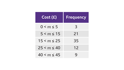
0·6, 2·1, 3·5, 0·8, 1·8
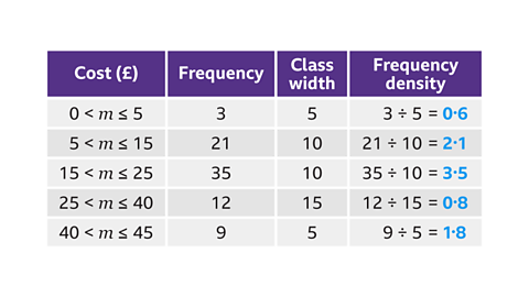
To calculate the ‘Frequency density’, divide the frequency by the class width.
- The histogram shows the time taken for participants to complete a fun run.
How many participants finished the race between 40 and 45 minutes?
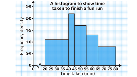
11
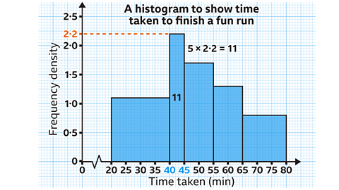
The frequency is calculated by multiplying the class width by the frequency density.
For the participants finishing the race between 40 and 45 minutes, the bar has a class width of five and frequency density of 2·2.
5 × 2·2 = 11
- The histogram shows the ages of members at a gym.
How many members in total does the gym have?
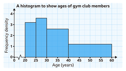
84 members
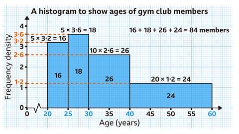
The frequencies for each bar are calculated by multiplying the class width by the frequency density.
- For the first bar: 5 × 3·2 = 16
- For the second bar: 5 × 3·6 = 18
- For the third bar: 10 × 2·6 = 26
- For the fourth bar: 20 × 1·2 = 24
Adding these frequencies, 16 + 18 + 26 + 24 = 84.
How to interpret a histogram
Sometimes a histogram might be presented with an incomplete frequency density scale. In this case additional information is provided, usually the frequency of one bar.
The additional information can be used either to reconstruct the frequency density scale or to allow a An area, often a square, used as a basis to measure and compare other areas. to be used, to calculate the frequencies for each bar.
Follow the worked example below
GCSE exam-style questions
- The histogram shows the mass of allotment carrots.
Given there are 25 carrots with a mass between 60 and 70 grams, work out the scale for the frequency density axis.
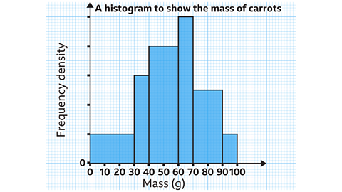
Each ten small squares is equivalent to 0·5.
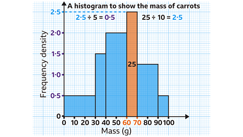
The 60 to 70 bar, representing 25 carrots, has a class width equal to 10.
To calculate the frequency density, divide the frequency by the class width.
25 ÷ 10 = 2·5
The height of this bar must correspond to 2·5 on the frequency density scale.
Between 0 and 2·5 there are 5 subdivisions of 10 small squares.
2·5 ÷ 5 = 0·5
This means 10 small squares are equal to 0·5.
- The histogram shows the mass of allotment carrots.
A carrot is chosen at random. What is the probability it has a mass of 40 grams or less?
Give the answer as a fraction in its simplest form.
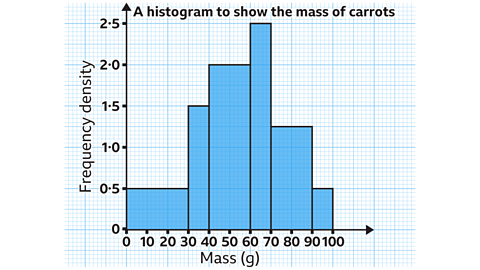
⁶⁄₂₅
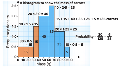
To work out the probability, first work out the frequencies represented by each bar.
- Calculate the frequencies for each bar by multiplying the class width by the frequency density.
- For the first bar: 30 × 0·5 = 15
- For the second bar: 10 × 1·5 = 15
- For the third bar: 20 × 2·0 = 40
- For the fourth bar: 10 × 2·5 = 25
- For the fifth bar: 20 × 1·25 = 25
- For the sixth bar: 10 × 0·5 = 5
- Adding these frequencies, 15 + 15 + 40 + 25 + 25 + 5 = 125.
There are 125 carrots altogether.
To work out the number of carrots that have a mass of 40 grams or less, add the frequencies of the first and second bars. 15 + 15 = 30
The probability of picking a carrot with a mass of 40 grams or less is ³⁰⁄₁₂₅. Dividing the numerator and denominator by five, the fraction simplifies to ⁶⁄₂₅.
- The histogram shows the length of telephone calls to a call centre.
There were 36 calls that lasted less than 10 minutes.
How many calls had a duration of 30 minutes and over?
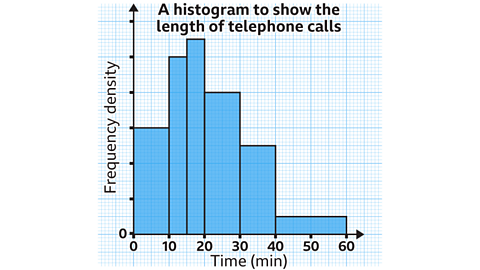
42 calls
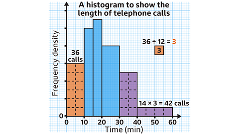
- Using the unit area method, the 0 to 10 bar, representing 36 calls, can be divided into 12 equal size squares, or unit areas.
36 ÷ 12 = 3
This means each unit area (5 small squares by 5 small squares) represents 3 calls.
- The interval between 30 and 60 minutes can be divided into 14 of these unit areas. Calculate the frequency by multiplying the number of unit areas by the number of calls each one represents.
14 × 3 = 42
There were 42 calls with a duration of 30 minutes and over.
How to find the median on a histogram
To estimate a A type of average calculated by finding the middle value of a set of numbers. If there are two middle numbers, the median is the mean of those two numbers. If there are 𝒏 values, the median is the ⁿ⁺¹⁄₂ th value. in a histogram, find a vertical line that chops the total area of the bars in half.
The line should have half of the area (or frequency) to the left of it and half the area to the right.
The value where this line intersects the 𝑥-axis is the median.
If a table with the frequencies is not provided, calculate these first.
Follow the worked example below
GCSE exam-style questions
- The histogram shows the length of 60 bags.
The frequency for each bar is provided.
Use the histogram to estimate the median length.
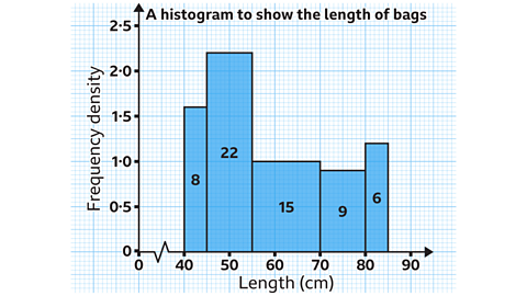
55 cm
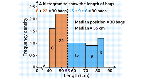
- To estimate the median, or the middle value, halve the total frequency, 60.
60 ÷ 2 = 30
A vertical line needs to be placed so that the area of the bars is equal to 30 on either side of the line.
The first two bars add up to a total frequency, or area, of exactly 30. The last three bars add up to a total frequency of exactly 30.
The vertical line, aligned with 55 cm on the horizontal axis, cuts the total area of the bars in half. The estimate for the median length of a bag is 55 cm.
- The histogram shows the mark in a music theory assessment for 800 people.
The frequency for each bar is provided.
Use the histogram to estimate the median mark.
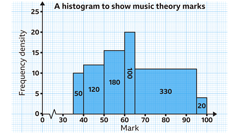
62·5 marks
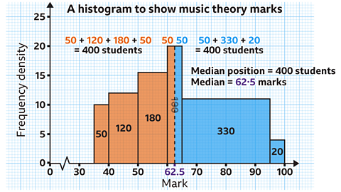
- To estimate the median, halve the total frequency, 800.
800 ÷ 2 = 400
A vertical line needs to be placed so that the area of the bars is equal to 400 on either side of the line.
The first three bars add up to a total frequency, or area, of 350. An additional area representing 50 students is needed from the fourth bar. The fourth bar represents 100 students. As a fraction, ½ of the bar is required.
The vertical line must split the fourth bar down the centre. This is aligned with 62·5 marks on the horizontal axis, leaving an area representing 400 students on either side of the line.
The estimate of the median is 62·5 marks.
- The histogram shows the height of 80 trees in a park.
Use the histogram to estimate the median height.
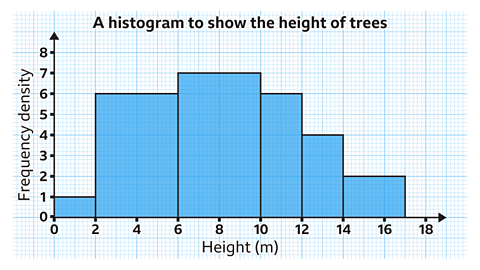
8 m
- To estimate the median, first work out the frequencies represented by each bar. Calculate these by multiplying the class width by the frequency density.
- For the first bar: 2 × 1 = 2
- For the second bar: 4 × 6 = 24
- For the third bar: 4 × 7 = 28
- For the fourth bar: 2 × 6 = 12
- For the fifth bar: 2 × 4 = 8
- For the sixth bar: 3 × 2 = 6
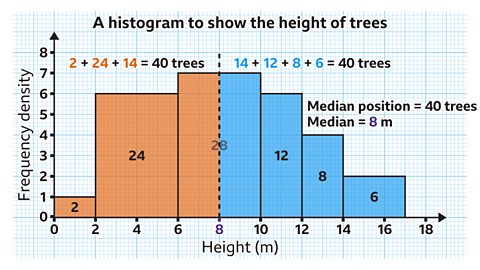
- The total frequency adds up to 80.
80 ÷ 2 = 40
A vertical line needs to be placed so that the area of the bars is equal to 40 on either side of the line.
The first two bars add up to a total frequency, or area, of 26. An additional area, representing 14 trees, is needed from the third bar. The third bar represents 28 trees. As a fraction, ½ of the bar is required.
The vertical line must split the third bar down the centre. This is aligned with 8 m on the horizontal axis, leaving an area representing 40 trees on either side of the line.
The estimate of the median is 8 metres.
Quiz – Higher – Histograms
Practise what you've learned about histograms with this quiz.
Now you've revised histograms, why not look at Higher – Solving problems using Venn diagrams?
More on Statistics
Find out more by working through a topic
- count5 of 7
- count6 of 7

- count7 of 7

- count1 of 7