Key points about cumulative frequency and box plots

Cumulative frequency graphs and box plots are two methods used to display Continuous data can take any value within a range. It is data which has been measured rather than counted, eg time, length, mass..
A cumulative frequency graph is used to estimate the A type of average calculated by finding the middle value of a set of numbers. If there are two middle numbers, the median is the mean of those two numbers. If there are 𝒏 values, the median is the ⁿ⁺¹⁄₂ th value. and calculate the A measure of spread that uses the central 50% of the dataset.. The interquartile range is calculated by finding the difference between the The value in a dataset that is the 75th percentile. and The value in a dataset that is the 25th percentile..
Box plots present the same data in a different way and can be used to make comparisons between two similar datasets.
Make sure you are confident in finding the median for a list of A collection of unprocessed information. when working with cumulative frequency graphs and box plots.
How to construct and interpret a cumulative frequency graph
Data is required to produce a cumulative frequency graph. The data should be provided in the form of a A table that organises large datasets into class intervals..
Creating a cumulative frequency graph
Add an additional column, if not provided, to the grouped frequency table. Label the column ‘Cumulative frequency’.
The cumulative frequency is an increasing total of all the frequencies. For each cell, add up the previous frequencies. The final value should match the total frequency.
Draw a horizontal axis. This should be a continuous number line. The values used to label the axis should match the numbers from the class intervals of the groups. Decide if you need to use a A symbol indicating a break in the scale on an axis. .
Draw a vertical axis. The vertical axis is always cumulative frequency. Choose an appropriate scale for this axis which includes the highest value in the cumulative frequency column.
Plot each data point. Each data point is plotted by using the value at the end of the class interval and the cumulative frequency.
The graph can be completed in one of two ways:
i. Join each consecutive point with straight lines. In this case this graph is called a cumulative frequency polygon.
ii. Draw a smooth curve passing through each point. In this case this graph is called a cumulative frequency curve.
Check you have labelled each axis correctly and give your cumulative frequency graph a title.
Follow the worked example below
GCSE exam-style questions

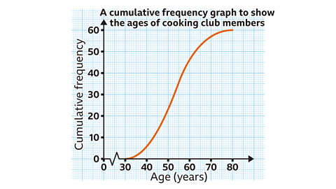
- The cumulative frequency graph shows information about the ages of 60 cooking club members.
Use the graph to estimate the median age of the members.
Median = 53 years
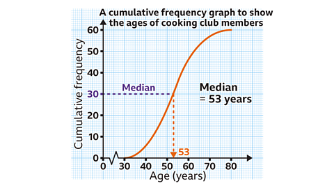
In this group of 60 members the middle value is the 30th member.
Find 30 on the cumulative frequency axis and follow the line across to the curve. Then, read down to the bottom axis to find the age.
The median age of the members is 53 years.
- The cumulative frequency graph shows information about the ages of 60 cooking club members.
Use the graph to estimate the interquartile range of the members.
IQR = 13·5 years
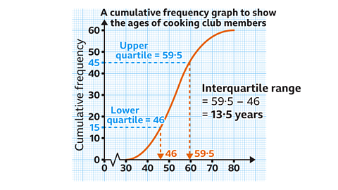
The lower quartile is the value at the one-quarter mark. For 60 members, this is the age of the 15th member.
The upper quartile is the value at the three-quarters mark. For 60 members, this is the age of the 45th member.
Lower quartile = 46 years
Upper quartile = 59·5 years
The IQR is calculated by subtracting the upper quartile and lower quartile.
IQR = 59·5 – 46 = 13·5 years
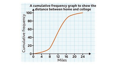
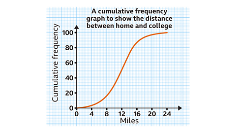
- This cumulative frequency graph shows information about the distance between the home and college of 100 students.
Use the graph to estimate the percentage of students that live more than 14 miles from their college.
28%
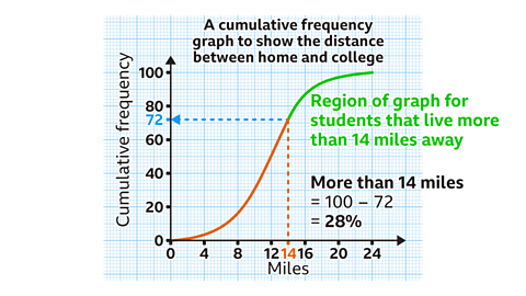
Find 14 miles on the horizontal axis and read up to the curve, then across to the cumulative frequency.
This corresponds to 72 students. Since the total is out of 100, this is equal to 72%.
This is an estimate of the percentage of students that live less than 14 miles from college.
To find the percentage of students that live more than 14 miles from college, subtract this from 100.
100 – 72 = 28
How to construct a box plot
A box plot (or box and whisker diagram) is another way of presenting the distribution of a continuous data set. In addition to showing the median and quartiles, it also displays the smallest and largest values.
The length of the box, which represents the A measure of spread that uses the central 50% of the dataset., shows how spread the central data is.
The horizontal scale below the box plot allows for the values to be accurately recorded or read.
Create a box plot from a list of raw data by ordering the numbers and identifying the median and quartiles.
Find the positions of the quartiles and median using the following formulae, where \(𝑛\) is the number of pieces of data:
- Lower quartile = \( \frac{1}{4} (𝑛 + 1) \)
- Median = \( \frac{1}{2} (𝑛 + 1) \)
- Upper quartile = \( \frac{3}{4} (𝑛 + 1) \)
Follow the worked example below
GCSE exam-style questions
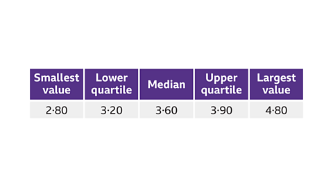
- The table shows information about the cost of lunches (£) of pupils at a school.
Draw a box plot to show this information.
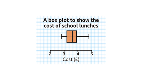
With all the necessary values provided, the box plot can be plotted.
Start by creating a horizontal scale, for example from 2 to 5. In this scale each small square represents 10 pence.
Then create the box, which has a length from the lower quartile, 3·20, to the upper quartile 3·90. The line for the median is at 3·60.
Add the ‘whiskers’ from the smallest value 2·80 to the box, and on the other side to the largest value, 4·80.
Remember to add an appropriate title.
- The masses (kg) of 11 sofas are recorded below.
49, 56, 57, 63, 67, 67, 71, 75, 81, 82, 93
Draw a box plot for this information.
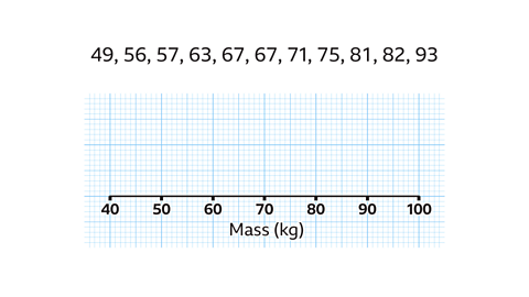
To create a box plot, identify the quartiles, the median and the smallest and largest values.
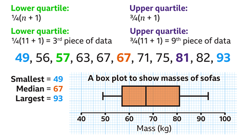
The numbers are already in ascending order. The smallest number is 49. The largest number is 93. The median, the number in the middle, is 67.
- To find the position of the quartiles, use the formulae \( \frac{1}{4} (𝑛 + 1) \) and \( \frac{3}{4} (𝑛 + 1) \), where \(𝑛\) is the number of pieces of data.
In this dataset there are 11 pieces of data, so \(𝑛 = 11\).
\( \frac{1}{4} (11 + 1) = 3 \)\( \frac{3}{4} (11 + 1) = 9 \)
The lower quartile is the 3rd piece of data, and equals 57.
The upper quartile is the 9th piece of data, and equals 81.
With all the necessary values identified the box plot can be plotted. Start with the box, which has a length from the lower quartile, 57, to the upper quartile 81. The line for the median is at 57.
Add the ‘whiskers’ from the smallest value 49 to the box, and on the other side to the largest value, 93.
Remember to add an appropriate title.
- The cumulative frequency graph shows information about the distance between home and college of 100 students.
The closest student lives 3·6 miles from college.
The furthest student lives 20·8 miles from college.
Using the graph, create a box plot for this information.
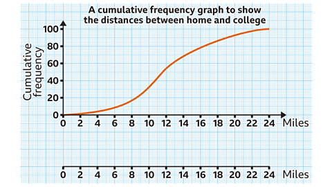
To create a box plot, first identify the quartiles and the median from the cumulative frequency graph.
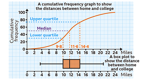
- In this question, with 100 students, the middle value is the distance to college for the 50th student. Find 50 on the cumulative frequency and read across to the curve, then down to the horizontal axis.
The median distance is 11·6 miles.
- The lower quartile is the value at the one-quarter mark. For 100 students, the lower quartile is the distance to college for the 25th student.
Lower quartile = 9·8 miles.
- The upper quartile is the value at the three-quarters mark. For 100 students, the upper quartile is the distance to college for the 75th student.
Upper quartile = 14·4 miles.
- With all the necessary values identified, the box plot can be plotted. Start with the box, which has a length from the lower quartile, 9·8, to the upper quartile, 14·4.
The line for the median is at 11·6.
- Add the ‘whiskers’ from the smallest value, 3·6, to the box, and on the other side to the largest value, 20·8. Remember to add an appropriate title.
Check your understanding
Using the median and interquartile range to make comparisons
For two sets of similar data, it is possible to draw two box plots on the same set of axes.
Comparisons can be made between the data, often by using the median and interquartile range.
For example, when comparing the data between the prices of flights that two airlines offer, a higher median would mean, on average, that the flights are more expensive. A smaller IQR means there is more consistency in the variation of prices.
When making a comparison, always quote numerical values and explain what they mean.
Find out more about making comparisons below
GCSE exam-style questions
- The box plots show the annual salaries of the workforce at two companies, White’s and Underwood’s.
On average, which company pays the higher salary?

Underwood's
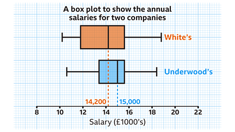
Using the median, White’s have a median salary of £14,200 and Underwood’s have a median salary of £15,000.
The median salary for Underwood’s is higher.
This means, on average, the company Underwood’s pays the higher salary.
- The box plots show the annual salaries of the workforce at two companies, White’s and Underwood’s.
Which company is more consistent with its salaries?
Underwood's
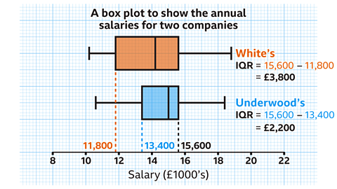
To work out which company is more consistent, use the interquartile range.
To calculate the IQR, subtract the lower quartile from the upper quartile.
The IQR for White’s is £3800.
The IQR for Underwood’s is £2200.
The IQR for Underwood’s is lower.
This means the employees at Underwood’s are more consistently paid.
- The box plots show the waiting times of patients for two doctors.
Which doctor is more consistent with their waiting times?
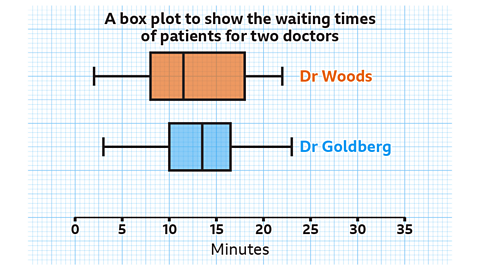
Dr Goldberg
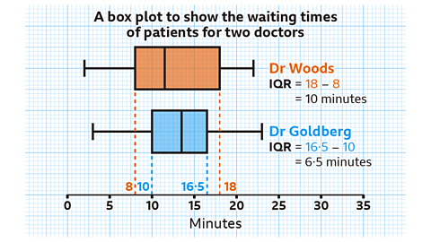
To work out which doctor is more consistent, use the interquartile range.
To calculate the IQR, subtract the lower quartile from the upper quartile.
The IQR for Dr Woods is 10 minutes.
The IQR for Dr Goldberg is 6·5 minutes.
The IQR for Dr Goldberg is lower.
This means the patients waiting to see Dr Goldberg have a more consistent wait time.
Quiz – Cumulative frequency and box plots
Practise what you've learned about cumulative frequency and box plots with this quiz.
Now you've revised cumulative frequency and box plots, why not look at tree diagrams?
More on Statistics
Find out more by working through a topic
- count4 of 7

- count5 of 7

- count6 of 7

- count7 of 7